Clustering from correlation matrix

Prerequisites for annotating the produced dendrogram

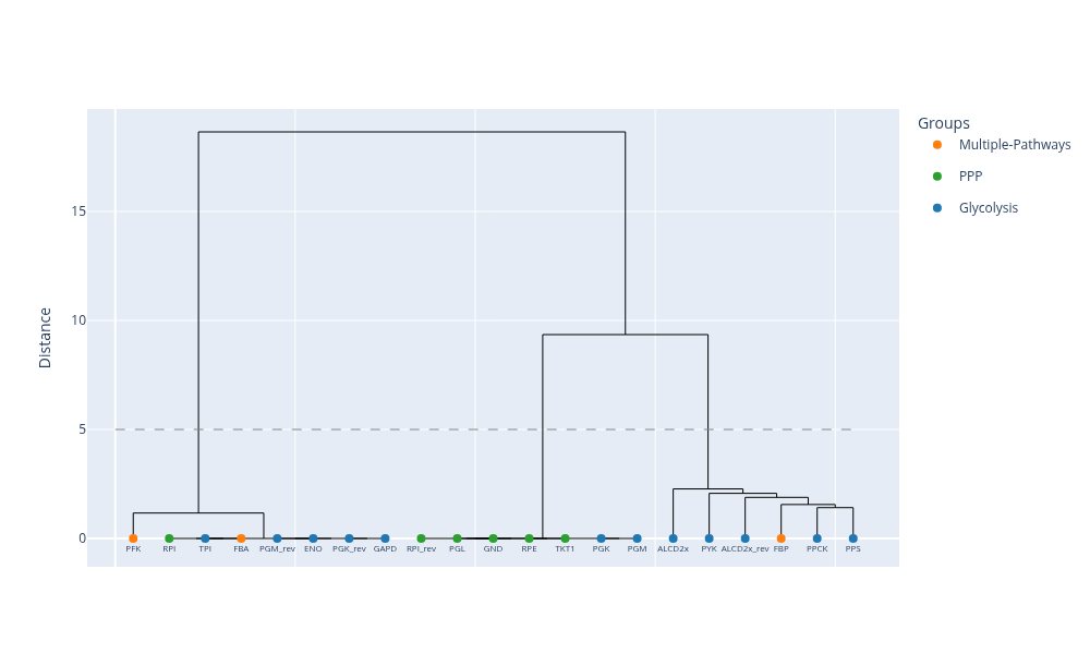
Suppose we have a correlation matrix produced from the correlated_reactions function, as shown in the previous section. After a split of the reversible reactions to separate forward and reverse reactions, we need to map the produced reverse reactions to their KEGG terms (identical term, as the forward reaction).

The dictionary_map_reverse_reaction_id_to_pathway function is used when we split bidirectional reactions to separate forward and reverse reactions. It maps the reverse reaction to the corresponding pathway (the one that the forward reactions maps to). It enriches the dictionary created from the dictionary_reaction_id_to_pathway function and we can annotate the produced dendrogram with pathway information.

• reaction_id_to_pathway_dict is a dictionary mapping reaction IDs (default-forward IDs) to pathway names

• for_rev_reactions is a list of the splitted reactions (forward ID is the default and reverse ID has the “_rev” suffix)

group_map_100 = dictionary_map_reverse_reaction_id_to_pathway(
    reaction_id_to_pathway_dict = bigg_to_pathway_dict, 
    for_rev_reactions = subset_extended_reactions_100)

print(group_map_100.get("PGM"))
print(group_map_100.get("PGM_rev"))

Glycolysis
Glycolysis

Hierarchical Clustering with Dendrogram Visualization

The default options to perform clustering in dingo-stats is the hierarchical clustering. This is a suggested method, however the user can procceed to clustering with any of the available methods, that are also presented in the next section.

The clustering_of_correlation_matrix function performs hierarchical clustering of the correlation matrix. It returns the dissimilarity_matrix (1sr arg.) calculated from the given correlation matrix, the integer labels (2nd arg.) corresponding to clusters and the clusters list (3rd arg.) which is a nested list containing reaction IDs grouped based on their cluster labels

• correlation_matrix is a numpy 2D array of a correlation matrix

• reactions is a list with the corresponding reaction IDs (must be in accordance with the order of rows in the correlation matrix)

• linkage is a string variable that defines the type of linkage. Available linkage types are: single, average, complete, ward.

• t is a float variable that defines a threshold that cuts the dendrogram at a specific height and produces clusters

• correction is a boolean variable that if True converts the values of the the correlation matrix to absolute values.

(dissimilarity_matrix,
labels,
clusters) = clustering_of_correlation_matrix(
    correlation_matrix = subset_mixed_correlation_matrix_100,
    reactions = subset_extended_reactions_100,
    linkage = "ward",
    t = 1.0,
    correction = False)

The plot_dendrogram function plots the dendrogram occured from hierarchical clustering

• dissimilarity_matrix is a dissimilarity matrix calculated from the clustering_of_correlation_matrix function

• reactions is a list with reactions IDs, that must be in accordance with the order of rows in the dissimilarity_matrix

• show_labels is a boolean variable that if True labels are shown in the x-axis

• t is a float variable that defines a threshold that cuts the dendrogram at a specific height

• linkage is a string variable that defines the type of linkage. Available linkage types are: single, average, complete, ward.

• group_map is a dictionary mapping reactions to pathways, produced from the dictionary_map_reverse_reaction_id_to_pathway function

• label_fontsize is an integer variable that defines the size for the plotted labels (reaction IDs)

• height is an integer variable that defines the height of the plot

• width is an integer variable that defines the width of the plot

• title is the title for the dendrogram plot

plot_dendrogram(
    dissimilarity_matrix = dissimilarity_matrix_100, 
    reactions = subset_extended_reactions_100, 
    show_labels = True, 
    t = 5, 
    linkage = "ward", 
    group_map = group_map_100,
    label_fontsize = 8,
    height = 600,
    width = 1000,
    title = "" )

Benchmarking with other clustering methods

In the clustering_of_correlation_matrix function we have implemented only the hierarchical (Agglomerative) clustering of the correlation matrix. However, other powerful clustering algorithms exist and we encourage users to test the different methods and decide which they are going to use.

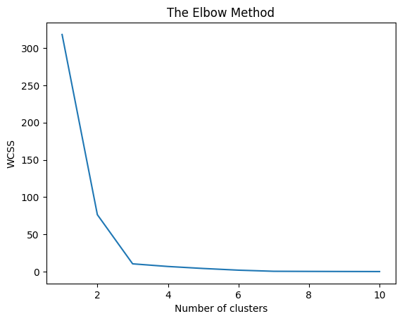
First, we start with the elbow method to find the ideal number of clusters, as some of the clustering algorithms used below use this as a parameter.

Here, we can see that n_clusers = 3, seems to produce better results

from sklearn.cluster import KMeans
import matplotlib.pyplot as plt

X = subset_mixed_correlation_matrix_100.copy()

wcss = []
for i in range(1, 11):
    kmeans = KMeans(n_clusters = i, init = 'k-means++',
                random_state = 42)
    kmeans.fit(X)
    wcss.append(kmeans.inertia_)
    
plt.plot(range(1, 11), wcss)
plt.title('The Elbow Method')
plt.xlabel('Number of clusters')
plt.ylabel('WCSS')
plt.show()

Benchmark across KMeans, AgglomerativeClustering, DBSCAN, HDBSCAN and SpectralClustering clustering methods with the Silhouette, Calinski-Harabasz and Davies-Bouldin scores, reveals which method produces better clusters

Here, we benchmark across these clustering methods and provide some metrics to give insights on clustering quality:

• Silhouette Score: Scores closer to 1 are better

• Calinski-Harabasz Score: Higher scores are better

• Davies-Bouldin Score: Lower scores are better

from sklearn.cluster import KMeans, AgglomerativeClustering, DBSCAN, SpectralClustering
import hdbscan
from sklearn.metrics import silhouette_score, calinski_harabasz_score, davies_bouldin_score
import numpy as np

X = subset_mixed_correlation_matrix_100.copy()
n_clusters = 3


kmeans_labels = KMeans(n_clusters=n_clusters, random_state=42).fit_predict(X)

agg_labels = AgglomerativeClustering(n_clusters=n_clusters, metric='euclidean', linkage='average').fit_predict(X)

dbscan = DBSCAN(eps=0.5, min_samples=n_clusters)
dbscan_labels = dbscan.fit_predict(X)

hdb = hdbscan.HDBSCAN(min_cluster_size=n_clusters)
hdbscan_labels = hdb.fit_predict(X)

spectral_labels = SpectralClustering(n_clusters=n_clusters, affinity='nearest_neighbors', random_state=42).fit_predict(X)


clusterings = {}

clusterings["KMeans"] = kmeans_labels
clusterings["Agglomerative"] = agg_labels
clusterings["DBSCAN"] = dbscan_labels
clusterings["HDBSCAN"] = hdbscan_labels
clusterings["Spectral"] = spectral_labels


def evaluate(X, labels, name):
    labels = np.array(labels)
    if len(np.unique(labels)) < 2 or np.all(labels == -1):
        print(f"\n{name}: Not enough clusters to evaluate.")
        return
    
    print(f"\n{name} Evaluation:")
    
    # Scores closer to 1 are better
    print(f"Silhouette Score:        {silhouette_score(X, labels):.4f}")
    # Higher scores are better
    print(f"Calinski-Harabasz Score: {calinski_harabasz_score(X, labels):.4f}")
    # Lower scores are better
    print(f"Davies-Bouldin Score:    {davies_bouldin_score(X, labels):.4f}")


for name, labels in clusterings.items():
    evaluate(X, labels, name)

KMeans Evaluation:
Silhouette Score:        0.8567
Calinski-Harabasz Score: 321.7593
Davies-Bouldin Score:    0.3168

Agglomerative Evaluation:
Silhouette Score:        0.8567
Calinski-Harabasz Score: 321.7593
Davies-Bouldin Score:    0.3168

DBSCAN Evaluation:
Silhouette Score:        0.8567
Calinski-Harabasz Score: 321.7593
Davies-Bouldin Score:    0.3168

HDBSCAN Evaluation:
Silhouette Score:        0.7811
Calinski-Harabasz Score: 207.2086
Davies-Bouldin Score:    0.3169

Spectral Evaluation:
Silhouette Score:        0.8567
Calinski-Harabasz Score: 321.7593
Davies-Bouldin Score:    0.3168

PCA and tSNE methods to reduce the dimensions of the correlation matrix

from sklearn.decomposition import PCA
from sklearn.manifold import TSNE

pca = PCA(n_components=2)
X_pca = pca.fit_transform(X)

X_tsne = TSNE(n_components=2, perplexity=3, random_state=42).fit_transform(X)

Define a function that will enable us to visualize clustering results

import numpy as np

def plot_clusters(embedding, labels, title, ax):
    labels = np.array(labels)
    unique_labels = np.unique(labels)
    for lab in unique_labels:
        mask = labels == lab
        ax.scatter(embedding[mask, 0], embedding[mask, 1], label=f"Cluster {lab}", s=80)
    ax.set_title(title)
    ax.legend()

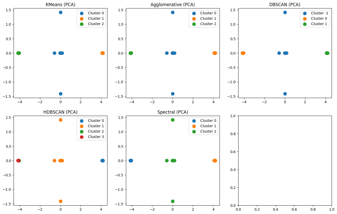
Visualize clustering results on a 2-dimensional space occured from the PCA algorithm

import matplotlib.pyplot as plt

fig, axes = plt.subplots(2, 3, figsize=(16, 10))
axes = axes.ravel()

for i, (name, labels) in enumerate(clusterings.items()):
    plot_clusters(X_pca, labels, f"{name} (PCA)", axes[i])

plt.show()

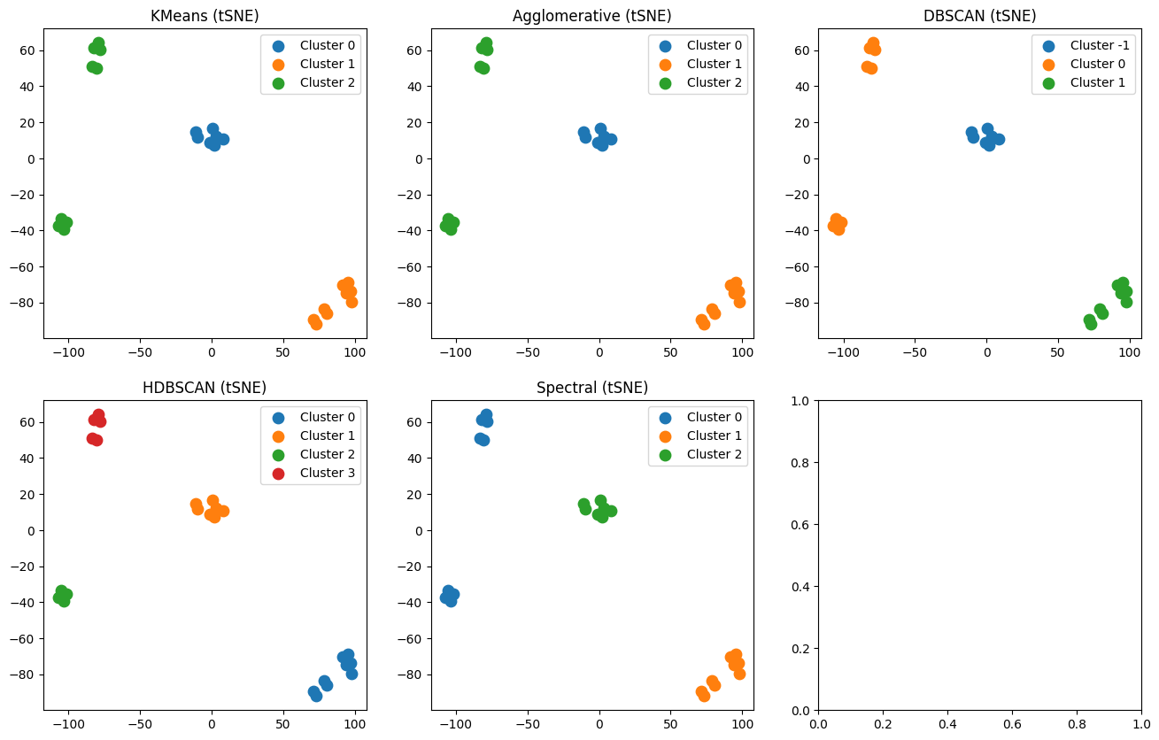
Visualize clustering results on a 2-dimensional space occured from the tSNE algorithm

import matplotlib.pyplot as plt

fig, axes = plt.subplots(2, 3, figsize=(16, 10))
axes = axes.ravel()

for i, (name, labels) in enumerate(clusterings.items()):
    plot_clusters(X_tsne, labels, f"{name} (tSNE)", axes[i])

plt.show()