Graphs from correlation matrix
Prerequisites for annotating the produced graph
The prerequisites for annotating the produced graph are the same as the ones described at the ## Prerequisites for annotating the produced dendrogram section of the Clustering from correlation matrix unit:
Make sure you have used the
correlated_reactionsfunction after split of the reversible reactions to separate forward and reverse reactionsCreate a dictionary from the
dictionary_map_reverse_reaction_id_to_pathwayfunction
Construct a graph
The construct_graph function creates a networkx graph from a linear correlation matrix or from both a linear correlation and a non-linear copula dependencies matrix. In this graph reactions are nodes and correlation values are edges. Users can also provide reaction-pathway mapping information in the group_map dictionary parameter and this will be saved in the graph for potential vizualization.
linear_correlation_matrixis a numpy 2D array corresponding to the linear correlation matrixnon_linear_correlation_matrixis a numpy 2D array (optional) corresonding to the non-linear copula dependencies matrixreactionsis a list of reaction names (ordered like matrix indices)remove_unconnected_nodesis a boolean variable that ifTrue, removes isolated nodescorrectionis a boolean variable ifTrue, absolute values of correlations (edges) are usedgroup_mapis a dictionary mapping reaction names to group names (pathways)
G100_full, pos100_full = construct_graph(
    linear_correlation_matrix = linear_correlation_matrix_100_full,
    non_linear_correlation_matrix = non_linear_correlation_matrix_100_full,
    reactions = extended_reactions_100,
    remove_unconnected_nodes = False,
    correction = False,
    group_map = group_map_100_full)
The compute_nodes_centrality_metrics function computes centrality measures for nodes (reactions) in the graph network: (A) Weighted degree centrality (normalized by number of nodes), (B) Betweenness centrality, © Clustering coefficient. Users should provide the full correlation matrices as input and not a subset based on certain reactions/pathways
Gis aNetworkXgraph with nodes and weighted edges; edges should have ‘weight’ and ‘source’ attributes
centrality_dict_100 = compute_nodes_centrality_metrics(
    G = G100_full)

print(centrality_dict_100.get("betweenness").get("PFK"))
print(centrality_dict_100.get("degree").get("PFK"))
print(centrality_dict_100.get("clustering").get("PFK"))
0.00809659410427305
0.22683071469001767
0.6179079858733398
Now, suppose we had created a second graph called G0_full from a different sampling dataset (corresponding to asking at least 0% of the biomass maximum value as an objective). The compare_node_centralities function compares node centralities between two centrality dictionaries for shared nodes and returns the difference by substracting the corresponding metric score of graph 2 (second argument) from graph 1 (first argument).
centrality_dict_1is a dictionary mapping node IDs to centrality values (first graph)centrality_dict_2is a dictionary mapping node IDs to centrality values (second graph)
sorted_betwenness_nodes = compare_node_centralities(
    centrality_dict_1 = centrality_dict_100.get("betweenness"),
    centrality_dict_2 = centrality_dict_0.get("betweenness"))

sorted_weighted_degree_nodes = compare_node_centralities(
    centrality_dict_1 = centrality_dict_100.get("degree"),
    centrality_dict_2 = centrality_dict_0.get("degree"))

print(dict(sorted_betwenness_nodes).get("CYTBD"))
print(dict(sorted_weighted_degree_nodes).get("CYTBD"))
0.1663975459581592
0.09272427760787
Both centrality metrics agree that the CYTBD node, has a higher centrality in the G100_full graph. Users are encouraged to examine the nodes with most extreme differences between the given graphs to get insights on the model’s behavior.
Visualize the constructed graph
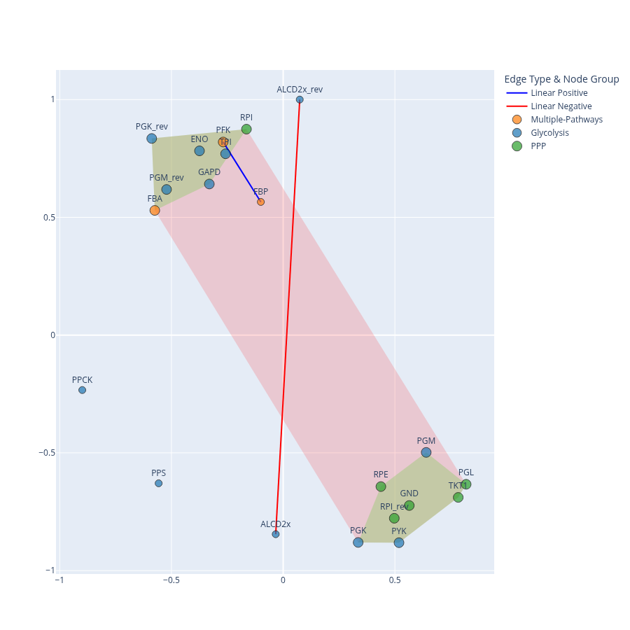
The plot_graph function a correlation-based networkx graph with multiple visual features including node annotations, edge styles, and clique-based shadowing. Here we are gonna plot a subset based on the 2 common pathays, we used in the previous sections: Glycolysis and Pentose Phosphate Pathway. The centrality metrics, provided in the centralities parameter should have occured from a full network and thus not be restricted to calculations from a sub-graph
Gis a NetworkX graph with nodes and weighted edges; edges should have ‘weight’ and ‘source’ attributesposis a dictionary of node positionsremove_clique_edgesis a boolean variable that ifTrue, edges within positive cliques and between negative cliques are removed and replaced with shadow areas (green for positive and red for negative)include_matrix2_in_cliquesis a boolean variable that ifFalse, only matrix1 (linear edges) is used for positive clique detection. IfTruecliques may be computed from a combination of linear corelations (matrix1) and copula dependencies (matrix2)min_clique_sizeis a minimum size for cliques to be considered (default = 5)shadow_edgesvisualization mode for clique shadows:None: no shadowspositive: show shadows around positive cliquesnegative: show shadows between cliques with negative edgesmixed: show both types of shadows
centralitiesis a dictionary containing precomputed centrality metrics
plot_graph(
    G = G100_glycolysis_ppp,
    pos = pos100_glycolysis_ppp,
    remove_clique_edges = True,
    include_matrix2_in_cliques = False,
    min_clique_size = 5,
    shadow_edges = "mixed",
    centralities = centrality_dict_100)